Mastering Excel Formula Referencing
How to reference formulas in Excel worksheet is crucial for efficient data manipulation. From basic arithmetic to complex calculations, understanding cell referencing, named ranges, and inter-worksheet formulas is key to unlocking Excel’s power. This guide will take you through the essentials, from simple relative references to advanced techniques like nested functions and error handling, empowering you to create dynamic and maintainable spreadsheets.
This comprehensive guide dives deep into the different types of referencing methods, from relative and absolute to mixed referencing, allowing you to tailor formulas to your specific needs. We’ll explore the benefits of named ranges, enhancing readability and simplifying complex formulas. Additionally, we’ll navigate the process of referencing cells across multiple worksheets, enabling you to connect data seamlessly from different parts of your workbook.
Introduction to Excel Formulas
Excel formulas are the backbone of data manipulation and analysis within the spreadsheet environment. They empower users to perform calculations, analyze data, and automate tasks with precision and efficiency. Formulas are essentially instructions that tell Excel what calculations to perform on specific data within a worksheet. They are essential for transforming raw data into actionable insights.Formulas are the driving force behind Excel’s capabilities, enabling users to derive meaningful information from their data.
From simple arithmetic calculations to complex statistical analyses, formulas streamline the process of extracting valuable insights. This section will explore the fundamental building blocks of Excel formulas, including their structure, types, and common operators.
Types of Excel Formulas
Excel formulas are categorized into various types, each designed for a specific purpose. Understanding these types is crucial for selecting the appropriate formula for a given task.
- Arithmetic formulas perform basic mathematical operations such as addition, subtraction, multiplication, and division. These are fundamental to many data analysis tasks, enabling users to perform calculations on numerical data.
- Logical formulas evaluate conditions and return a TRUE or FALSE result. These are vital for conditional formatting, filtering data, and creating complex decision-making processes in spreadsheets. For instance, an Excel formula can determine if a student’s grade is above or below a certain threshold.
- Text formulas manipulate text strings. These formulas are used to extract specific characters, concatenate strings, or perform searches within text data. Imagine extracting names from a list of customer data, or creating labels based on the customer’s location.
- Date/Time formulas work with dates and times, allowing for calculations and comparisons related to durations, intervals, and other date-related operations. A common example is calculating the number of days between two dates.
Formula Structure
Excel formulas always begin with an equals sign (=). This tells Excel that the subsequent characters constitute a formula, not just text. Following the equals sign, formulas consist of cell references, operators, and functions. Cell references indicate the cells containing the data to be used in the calculation. Operators define the specific mathematical or logical operations to be performed.
Functions are predefined formulas that perform specific tasks.
Example: =A1+B1
This formula adds the values in cells A1 and B1. A1 and B1 are cell references, “+” is the addition operator.
Common Excel Operators
The following table Artikels the most commonly used operators in Excel formulas:
| Operator | Description | Example |
|---|---|---|
| + | Addition | =A1+B1 |
| – | Subtraction | =A1-B1 |
| * | Multiplication | =A1*B1 |
| / | Division | =A1/B1 |
| ^ | Exponentiation | =A1^2 |
| & | Concatenation (joining text) | =”Hello” & ” ” & “World” |
| = | Equal to | =A1=B1 |
| <> | Not equal to | =A1<>B1 |
| > | Greater than | =A1>B1 |
| < | Less than | =A1 |
| >= | Greater than or equal to | =A1>=B1 |
| <= | Less than or equal to | =A1<=B1 |
Referencing Cells in Formulas
Excel formulas often rely on data from specific cells within the worksheet. Understanding how to reference these cells is crucial for creating dynamic and reusable calculations. Proper referencing allows formulas to adapt to changes in the underlying data without manual adjustments.Formulas in Excel can reference cells in various ways, each with distinct behavior when copied or modified. These methods, relative, absolute, and mixed references, determine how cell addresses are treated within the formula.
Relative References
Understanding how relative references behave when copied is essential for creating adaptable formulas. When a formula containing a relative reference is copied to a different cell, the cell references within the formula adjust based on the new location. This dynamic behavior allows the formula to automatically calculate values from corresponding cells in the new position.
- Consider a formula in cell A2 that calculates the difference between the value in A1 and B1. If this formula is copied to cell B2, the formula in B2 will adjust to calculate the difference between B1 and C1. The relative references have shifted one column to the right.
- For instance, if cell A1 contains 10, cell B1 contains 5, and the formula in A2 is `=A1-B1`, the result will be 5. Copying this formula to B2 results in the formula `=B1-C1`, and the outcome will depend on the values in B1 and C1.
Absolute References
Absolute references provide a way to maintain a constant cell reference when copying a formula. They are essential for calculations that need to consistently use the same cell, regardless of where the formula is placed. Absolute references are marked with a dollar sign ($) preceding the column and row designator (e.g., $A$1).
- If a formula in cell A2 uses an absolute reference to cell A1, like `=$A$1`, copying it to B2 will not change the reference; it will remain `=$A$1`. This ensures that the formula always uses the data from cell A1, irrespective of its position.
- Example: If cell A1 contains a company’s fixed overhead cost, say 100, and the formula in A2 is `=B1*$A$1`, calculating the cost of goods for the items in column B, then copying this formula to B2 will result in the formula `=C1*$A$1`. The formula will still use the value in A1.
Mixed References
Mixed references combine elements of relative and absolute references. They offer flexibility in maintaining some aspects of the reference while allowing other parts to adjust. A mixed reference can be either a row-relative column-absolute reference (e.g., $A1) or a column-relative row-absolute reference (e.g., A$1).
- A formula in cell A2 using a mixed reference, like `=A$1`, will adjust the column reference when copied to B2 but maintain the row reference to cell A1. The formula will become `=B$1`. This type of reference is useful when you want to use a specific row from a column consistently across various calculations.
- If a formula in cell A2 is `=$A1`, when copied to B2, it becomes `=$B1`. This type of reference keeps the column fixed, but the row changes, useful for using a specific column consistently across various rows.
Comparison Table
| Reference Type | Formula | Behavior when copied to B2 |
|---|---|---|
| Relative | =A1-B1 | =B1-C1 |
| Absolute | =$A$1 | =$A$1 |
| Row Relative, Column Absolute | =A$1 | =B$1 |
| Column Relative, Row Absolute | =$A1 | =$B1 |
Using Named Ranges
Excel’s named ranges offer a powerful way to enhance the readability, maintainability, and overall efficiency of your spreadsheets. Instead of using cryptic cell references like `$A$1` or `B2`, you can give descriptive names to ranges of cells, making your formulas more understandable and easier to manage, especially in complex spreadsheets. This is a key feature for collaborative work, where team members can easily comprehend and modify formulas without needing extensive context.Named ranges simplify formulas by allowing you to refer to a block of data using a meaningful name rather than its location.
This dramatically improves the clarity of formulas, particularly when dealing with large datasets or multiple calculations. Furthermore, modifying the data in a named range automatically updates all formulas referencing it, saving time and reducing the risk of errors.
Defining Named Ranges
Defining a named range involves associating a descriptive name with a specific cell range. This process is straightforward and easily integrated into your Excel workflow. To define a named range, select the range of cells you want to name. Next, go to the “Formulas” tab and click on “Define Name”. In the “New Name” dialog box, enter a name for the range.
The name should be concise, descriptive, and reflect the data contained in the range. For example, if the range contains sales data for the month of January, a suitable name would be “JanuarySales”. Once you’ve entered the name, click “OK.”
Using Named Ranges in Formulas
Once you’ve defined a named range, you can use it directly within your formulas. This substitution makes your formulas more understandable and easier to maintain. Instead of referencing cells by their coordinates, you can reference the named range by its name. For instance, if you have a named range called “JanuarySales” covering cells A1:A10, you can use it in a formula like `=SUM(JanuarySales)`.
This formula will calculate the sum of the values in the named range.
Example Demonstrations
Let’s consider a scenario where you’re tracking sales data. You have a column (Column A) for product names and a column (Column B) for corresponding sales figures. Suppose you want to calculate the total sales for a specific product. Instead of using `=SUM(B2:B10)`, you can define a named range “ProductSales” for the range of sales figures for the product.
Then, your formula would become `=SUM(ProductSales)`, which is significantly clearer.
Comparison of Cell References and Named Ranges
| Feature | Cell References | Named Ranges |
|---|---|---|
| Formula Clarity | Can be cryptic, especially for complex formulas. | Highly readable and descriptive, enhancing understanding. |
| Maintainability | Difficult to update if the referenced cells change position. | Easy to update as the referenced range changes. |
| Collaboration | Requires understanding of cell locations for modification. | Enables team members to understand and modify formulas without needing extensive context. |
| Example | `=SUM(B2:B10)` | `=SUM(ProductSales)` |
Working with Multiple Worksheets
Excel’s power often lies in its ability to manage data across multiple worksheets. This capability is invaluable for organizing large datasets, creating interconnected reports, and streamlining complex calculations. Understanding how to reference cells and ranges in different worksheets is a fundamental skill for leveraging Excel’s full potential.
Referencing Cells in Formulas from Different Worksheets
Formulas can effortlessly incorporate data from various worksheets within a workbook. This facilitates the linking of related information and streamlined analysis.
Referencing Cells in Another Worksheet Using the Worksheet Name
To reference a cell in another worksheet, you prepend the worksheet name followed by an exclamation mark (!) to the cell reference. This explicit method ensures unambiguous identification of the target cell.For example, if Sheet2 contains data in cell B3, you would reference it in Sheet1 as `Sheet2!B3`. This creates a static link; if Sheet2 is renamed, the formula in Sheet1 will need to be updated.
Using the INDIRECT Function for Dynamic Referencing
The `INDIRECT` function offers a dynamic alternative to referencing cells in other worksheets. It takes a text string representing the cell reference as an argument. This method is crucial when the worksheet name or cell address might change.
`=INDIRECT(“Sheet”&SheetNum&”!A1″)`
In this example, `SheetNum` is a cell containing the sheet number. If `SheetNum` contains “2”, the formula dynamically references cell A1 in Sheet2. This is particularly helpful when creating automated reports where worksheet names or locations change.
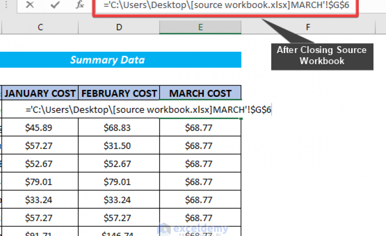
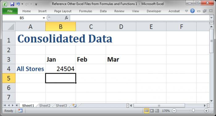
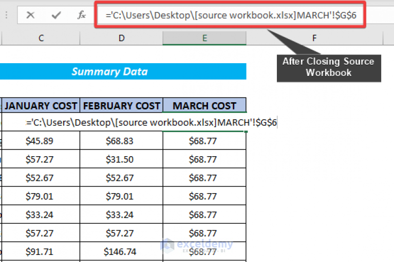
Demonstrating External Links from Another Sheet
Consider a scenario where you have sales data in a separate sheet. You might need to calculate the total sales across all regions. Linking the summary sheet to the sales data eliminates the need to manually copy and paste data, reducing errors and enhancing data consistency. The link is established using the worksheet name, followed by the cell address.
Step-by-Step Procedure to Create Formulas Referencing Cells in Another Worksheet
To create a formula referencing cells in another worksheet, follow these steps:
- Open the worksheet where you want to create the formula.
- Click on the cell where you want the formula to appear.
- Type the `=` sign to initiate the formula.
- Type the worksheet name, followed by an exclamation mark (!), and the cell reference.
- For example, if you want to reference cell B3 in Sheet2, type `Sheet2!B3`.
- Press Enter to complete the formula.
This procedure ensures that the formula correctly references the intended cell in the specified worksheet. Consistency and accuracy are critical in such formulas, especially when dealing with large datasets or automated calculations.
Advanced Formula Techniques: How To Reference Formulas In Excel Worksheet
Excel formulas are powerful tools, but their true potential unlocks when you combine multiple functions. Mastering advanced techniques like nested formulas, conditional logic, and array formulas allows you to create sophisticated spreadsheets capable of handling complex calculations and data analysis. These techniques empower you to automate tasks, extract insights, and build robust models.
Nested Formulas
Nested formulas involve placing one formula inside another. This powerful technique lets you perform complex calculations by combining different functions. It’s like having a series of instructions within a single command, making formulas more versatile and adaptable to intricate situations.
Consider a scenario where you need to determine a discount based on different criteria. A simple formula might handle a single condition, but a nested formula can incorporate multiple checks, such as quantity thresholds and product types, to calculate the precise discount. This complexity allows for much more nuanced results compared to simpler formulas.
Example:=IF(A1>100, B1*0.1, IF(A1>50, B1*0.05, 0))
This formula first checks if the value in cell A1 is greater than 100. If true, it applies a 10% discount to the value in cell B1. Otherwise, it checks if A1 is greater than 50. If true, it applies a 5% discount. Otherwise, it returns 0.
This example demonstrates how nested IF statements can cater to multiple conditions.
Conditional Logic with IF
The IF function is a cornerstone of conditional logic in Excel. It allows you to perform different calculations or actions based on specific conditions. Its versatility enables you to create formulas that respond dynamically to varying data.
For instance, you might need to flag sales exceeding a target or identify customers who meet certain criteria. The IF function is ideal for these scenarios, as it enables you to set up the calculations to match your needs, adapting to changing circumstances.
Example:=IF(A1>100,”Above Target”,”Below Target”)
This formula checks if the value in cell A1 is greater than 100. If it is, it returns the text “Above Target”; otherwise, it returns “Below Target”. This demonstrates the ability to return different outputs based on different conditions.
Error Handling with IFERROR
In real-world data, errors can arise from various sources, like missing data or incorrect formulas. The IFERROR function is crucial for handling these potential issues gracefully. It ensures that your formulas don’t crash or produce meaningless results when encountering errors.
This function allows you to anticipate potential problems, preventing disruptions in your workflow and providing more reliable results. Instead of displaying an error message, it can return a custom value, a blank cell, or a more appropriate calculation.
Example:=IFERROR(A1/B1, “N/A”)
This formula attempts to divide the value in cell A1 by the value in cell B1. If the division results in an error (e.g., division by zero), it returns the text “N/A” instead of the error. This ensures your spreadsheet functions smoothly even when encountering unexpected data.
Array Formulas
Array formulas perform calculations on multiple cells simultaneously, offering a powerful way to process large datasets. They excel in situations where you need to apply a function to an entire range of cells or perform calculations based on multiple criteria.
Imagine needing to calculate the average of all values in a column that meet a specific condition. Array formulas make this streamlined and efficient. You can use array formulas to work with entire columns or rows, allowing you to process data more effectively.
| Data | Description |
|---|---|
| =SUM(IF(A1:A10>10,A1:A10)) | This array formula calculates the sum of all values in the range A1:A10 that are greater than 10. |
This example demonstrates the power of array formulas in efficiently handling multiple conditions across a range of cells. This makes them very valuable for complex data analysis and automation tasks in spreadsheets.
Troubleshooting Formula Errors

Excel formulas are powerful tools, but errors can creep in. Knowing how to identify and fix these errors is crucial for accurate results. This section dives into common formula errors, their causes, and effective troubleshooting techniques.Common Excel formula errors often disrupt the entire worksheet’s calculations. Understanding their causes is essential to prevent further issues and ensure reliable data analysis.
This guide will not only show you how to identify these errors but also demonstrate practical methods to correct them and enhance your overall Excel proficiency.
Identifying Common Formula Errors
Knowing the telltale signs of errors is the first step in troubleshooting. Excel displays specific error codes, each with a distinct meaning. These error codes, often starting with a “#”, provide valuable clues to the source of the problem.
- #VALUE! This error arises when a function receives an incorrect data type. For example, trying to perform mathematical operations on text strings. If a function expects a number but receives text, Excel will display #VALUE!.
- #REF! This error indicates a reference to a cell that no longer exists. Perhaps you deleted a cell or shifted data, causing the formula to point to a void. Check all cell references in your formula.
- #DIV/0! This error results from dividing a number by zero. Excel cannot perform this operation, and the error code appears. Ensure that the denominator in your formula is never zero.
- #NAME? This error indicates that Excel cannot recognize a name or function within the formula. Double-check the spelling and ensure the function exists.
Causes of Formula Errors
Formula errors are often the result of simple oversights or mistakes.
- Typos A simple typo in a function name or cell reference can cause an error. Double-check all entries for correctness.
- Incorrect Data Types Functions operate on specific data types. Mismatched types lead to #VALUE! errors. For instance, using a text string where a number is expected.
- Circular References Formulas referencing themselves in a loop will result in an infinite calculation cycle. Be wary of formulas that reference each other in a chain.
- Missing Parentheses Unbalanced parentheses can disrupt the order of operations, leading to calculation errors.
Fixing Formula Errors
Once you’ve identified the error, the next step is to fix it.
- Review Formula Syntax Carefully examine the formula for any typos or incorrect syntax.
- Check Data Types Ensure that the data in the referenced cells matches the expected data type for the function.
- Verify Cell References Double-check all cell references in the formula. Ensure the cells still exist.
- Identify Circular References If a circular reference is detected, adjust the formula to avoid the loop.
Tracing Formula Errors
Tracing formula errors involves stepping through the calculation process to find the source of the problem. Excel’s built-in tools make this process easier.
- Formula Auditing Tools Excel provides tools to trace precedents and dependents of a formula. These tools help you understand how a formula interacts with other cells.
- Evaluate Formula Use the Evaluate Formula feature to step through each calculation step, observing the values and the formula’s impact on the cells.
- Step-by-Step Evaluation Evaluate the formula step-by-step to observe the intermediate calculations and pinpoint the point where the error occurs.
Common Excel Formula Errors and Resolutions
| Error | Cause | Resolution |
|---|---|---|
| #VALUE! | Incorrect data type in the formula | Verify the data type of cells referenced in the formula. Correct any mismatches. |
| #REF! | Invalid cell reference | Correct any invalid cell references in the formula. |
| #DIV/0! | Division by zero | Ensure the denominator in the division operation is not zero. |
| #NAME? | Invalid function or name | Check the spelling of the function or name in the formula. |
Best Practices for Formula Design
Excel formulas, while powerful, can become complex and difficult to understand and maintain if not designed carefully. Following best practices ensures formulas remain readable, efficient, and easily debugged, saving you time and frustration in the long run. Clear, well-structured formulas are essential for collaborative work and long-term project sustainability.
Importance of Formula Readability
Formulas should be written in a way that anyone who needs to understand or modify them can easily do so. Avoid cryptic abbreviations and overly complex nested structures. Prioritize clarity over brevity, especially when dealing with formulas that might need modification in the future. Using meaningful names for ranges and cells is crucial for this. For example, instead of `=A1+B2`, use `=SalesQ1+ExpensesQ1` if those cells represent those metrics.
Strategies for Creating Clear and Maintainable Formulas
Breaking down complex calculations into smaller, more manageable formulas is crucial. Use intermediate variables to store intermediate results. This not only improves readability but also allows for easier debugging and modification. This approach also enhances formula efficiency. For example, if you have a complex calculation involving multiple steps, calculate the individual steps in separate cells and then use these intermediate results in the final formula.
This approach reduces the likelihood of errors and makes modifications straightforward.
Use of Comments in Formulas
Comments are essential for documenting the purpose and logic of a formula. They clarify the reasoning behind specific calculations and help others (and your future self) understand the formula’s function. Excel allows you to add comments directly to cells containing formulas. For example, a comment like “//Calculate total sales for Q1” can significantly enhance the clarity of a formula calculating total sales.
This makes debugging and future modifications much easier.
Impact of Formula Complexity on Performance, How to reference formulas in excel worksheet
Complex formulas involving many nested functions or extremely large ranges can negatively impact the performance of your Excel workbook. Repeated calculations and large data sets can lead to significant delays in loading and recalculating the worksheet. Avoid excessively complex formulas, and if possible, use simpler formulas or external data sources to accomplish the same task. For example, avoid using 10 nested IF statements when you can achieve the same logic with a lookup table.
This can be extremely beneficial for spreadsheets with substantial data sets.
Checklist of Best Practices for Designing Efficient Formulas
- Use meaningful names for ranges and cells. This significantly enhances formula readability and maintainability. Avoid cryptic abbreviations or single-letter names.
- Break down complex formulas into smaller, manageable steps. This approach makes the formula more understandable and less error-prone. Calculate intermediate results in separate cells to isolate and validate each step.
- Use intermediate variables to store intermediate results. This enhances formula readability and maintainability. Using temporary variables clarifies the formula’s logic and improves future modification.
- Add comments to formulas to document their purpose and logic. Use comments to explain the rationale behind specific calculations. This aids in debugging and understanding the formula’s function.
- Avoid excessively nested formulas. Excessive nesting can lead to slower calculation times and reduced formula readability. If possible, use alternative approaches such as lookup tables or helper columns.
- Use appropriate functions for the task. Using the right function for the job significantly improves formula efficiency and readability. Choose functions that are designed for the specific calculation, reducing redundant steps.
- Optimize formula structure for performance. Evaluate the potential impact of formula complexity on calculation times. Avoid unnecessary calculations and use more efficient functions to enhance spreadsheet performance.
Concluding Remarks
In conclusion, mastering how to reference formulas in Excel worksheets is a journey of discovery. By understanding relative, absolute, and mixed references, utilizing named ranges, and navigating inter-worksheet formulas, you can significantly improve your spreadsheet’s efficiency and readability. This comprehensive guide equips you with the knowledge to tackle any Excel formula challenge, from basic calculations to complex data analyses.
Now go forth and conquer your spreadsheets!